Over on Twitter I asked whether anyone knew of literature which showed that parliaments which were more representative with respect to one characteristic were also more representative in terms of other characteristics.

I didn’t get any replies, so I’m going to try and answer my question here.

Descriptive representation of what?

The first problem in studying descriptive representation is giving an answer to the question “descriptive representation of what?”

I think most studies of descriptive representation have involved gender as the primary or sole characteristic. The second most popular characteristic in the literature is probably race: this is particularly true of the literature on descriptive representation in the United States.

These two characteristics are very different. Gender is (almost always in the case of elected representatives) easily observed, and in almost all national populations the proportion of men and women is within a couple of percentage points of fifty percent. (Exceptions include societies with large migrant male populations).

The race (or ethnicity) of elected representatives is much harder to observe or infer, and in some cases we lack any population statistics on ethnicity. Looking at you, France.

Thanks to some recent work, much of it by Daniel Stockemer and Aksel Sundström, age has become an increasingly studied characteristic.

Because statistics on age are readily available, and because age is cross-nationally comparable (now that Koreans have agreed with the rest of the world), in this post I’ll be looking at descriptive representation in terms of gender and age. I’ll be assessing representativeness with respect to these characteristics separately (rather than investigating the intersection of the two), and asking whether legislatures which have greater levels of descriptive representation with respect to gender also have greater levels of descriptive representation with respect to age group.

The data

Stockemer and Sundström have published a data-set which includes information on

the percentage of MPs who are female;
the percentage of MPs in three exclusive age categories (under 40, 41 to 60, and 60 plus)
The ratio of the percentage of MPs in these categories to the corresponding population percentage (their Age Representation Index)

Using information on the Age Representation Index, we can calculate the proportion of the population in each of these three age categories.

We can then calculate inequalities of representation by

Taking the population proportion for each age or gender group
Subtracting the proportion of MPs in that age or gender group
Squaring the result (to make negative values positive)
Calculating the sum of squares, and then
Taking the square root to return this measure to the original scale.

I do that in the code below. I begin by reading in the data, and removing some observations which have incomplete or inaccurate data.

suppressPackageStartupMessages(library(tidyverse))
### data.csv is downloaded from http://www.warpdataset.com/download.php
warp <- read.csv("data.csv")
### Restrict just to cases where we have ARIs
nrow(warp)

[1] 871

warp <- warp |>
    filter(!is.na(Age.Representation.Index.40.or.under..ARI.40.)) |>
    filter(!is.na(Age.Representation.Index.41.to.60..ARI.41.to.60.)) |>
    filter(!is.na(Age.Representation.Index.61.or.over..ARI.61.plus.))
nrow(warp)

[1] 817

### Exclude cases where proportions exceed 100%
### Check no proportions exceed 100
warp$sum_totals <- rowSums(warp[,c("Percent.MPs.aged.40.or.under",
                                   "Percent.MPs.aged.41.to.60",
                                   "Percent.MPs.aged.61.or.over")])

nrow(warp)

[1] 817

warp <- warp |>
    filter(sum_totals <= 101) |>
    filter(sum_totals > 95)
nrow(warp)

[1] 702

I then calculate the population proportions for each age group using the Age Representativeness Index (ARI) The ARI is calculated by taking the proportion for MPs and dividing by the population proportion, so to reverse this, we need to get the proportion for MPs and divide by the ARI.

warp <- warp |>
    mutate(pop_sub_40 = Percent.MPs.aged.40.or.under /
               Age.Representation.Index.40.or.under..ARI.40.,
           pop_41_to_60 = Percent.MPs.aged.41.to.60 /
               Age.Representation.Index.41.to.60..ARI.41.to.60.,
           pop_61plus = Percent.MPs.aged.61.or.over /
               Age.Representation.Index.61.or.over..ARI.61.plus.)

I can then calculate mean root squared differences – analogous to measures of disproportionality for votes and seats – for age and gender. I do so assuming that the gender balance is 50:50 in all cases.

warp <- warp |>
    mutate(disp_gender = sqrt(((Percent.female.MPs - 50)^2 +
                              ((100 - Percent.female.MPs) - 50)^2)/2))

warp <- warp |>
    mutate(disp_age = sqrt((pop_sub_40 - Percent.MPs.aged.40.or.under) ^ 2 +
               (pop_41_to_60 - Percent.MPs.aged.41.to.60) ^ 2 +
               (pop_61plus - Percent.MPs.aged.61.or.over) ^ 2)/2)

With all of this done, we can now ask – are legislatures which are more (descriptively) representative with respect to gender also more descriptively representative with respect to age group?

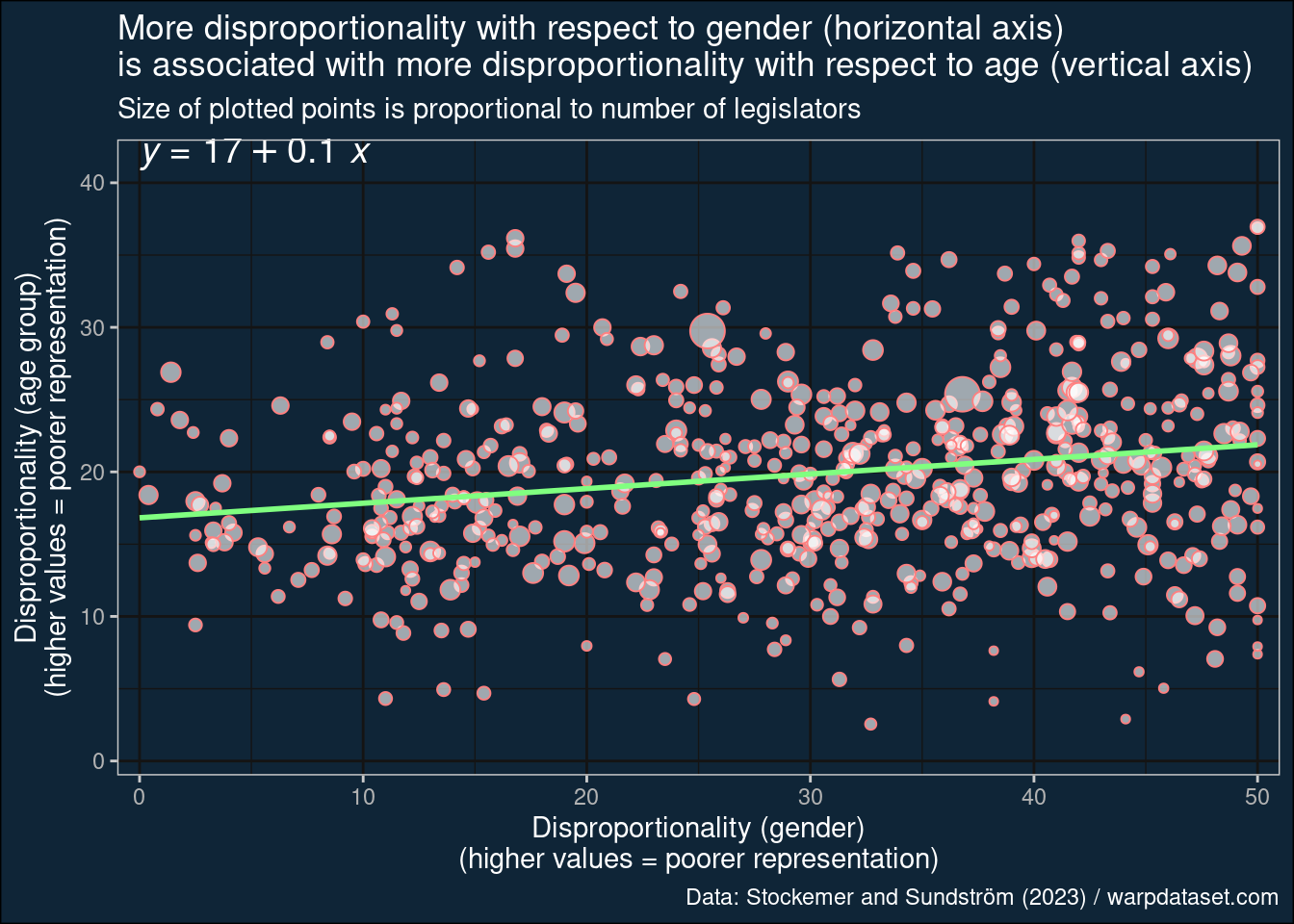
Let’s do this by plotting a scatterplot and overlaying a regression line. Remember, the quantities we’re plotted are disproportionalities, so higher values is worse.

library(ggdark)
library(ggpubr)
ggplot(warp, aes(x = disp_gender,
                 y = disp_age)) +
                 ## weight = Number.of.MPs)) +
    scale_x_continuous("Disproportionality (gender)\n(higher values = poorer representation)",
                       limits = c(0, NA), expand = c(0, 1)) +
    scale_y_continuous("Disproportionality (age group)\n(higher values = poorer representation)",
                       limits = c(0, NA), expand = c(0, 1)) +
    scale_size_continuous(guide = "none") + 
    geom_point(aes(size = Number.of.MPs),
               shape = 21,
               fill = "#FFFFFF99",
               colour = "#ff8080") +
    geom_smooth(method = "lm", colour = "#80ff80", se = FALSE) +
    stat_regline_equation(label.x = 0, label.y = 42, size = 5) + 
    dark_theme_bw() +
    theme(plot.background = element_rect(fill = "#0f2537"),
          panel.background = element_rect(fill = "#0f2537"),
          legend.background = element_rect(fill = "#0f2537")) +
    labs(title = "More disproportionality with respect to gender (horizontal axis)\nis associated with more disproportionality with respect to age (vertical axis)",
         subtitle = "Size of plotted points is proportional to number of legislators",
         caption = "Data: Stockemer and Sundström (2023) / warpdataset.com")

As you can see from the Figure, the worse the representation of gender (i.e., the further we move to the right on the plot), the worse also the representation of age (i.e., the further we move to the top of the plot).

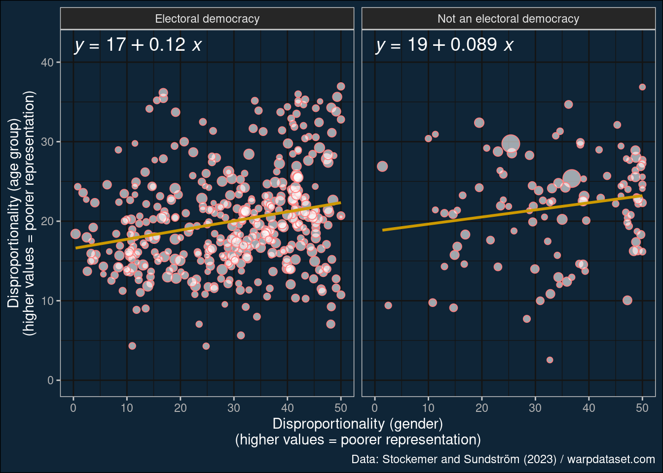
This association is not particularly strong (\(r = 0.2\)), but this is perhaps what we would expect given that our sample is a wildly heterogeneous convenience sample, and given that we haven’t restricted it to countries where we expect the same mechanisms (prejudiced voters whose votes are translated into distributions of seats) to operate. Maybe if we restricted the analysis to democracies we’d see a clearer trend. So let’s try that now.

Specifically, let’s join this data with V-Dem data, using their measure of electoral democracy v2x_polyarchy, and splitting countries based on whether their value is greater than 0.5 (“electoral democracies”) or lower than 0.5 (“not an electoral democracy”). The choice of cut-off isn’t material, and other cut-offs can work as well.

library(vdemdata)
data("vdem")
warp <- left_join(warp,
                  vdem |> dplyr::select(country_text_id, year,
                                        v2x_polyarchy),
                  by = c("Country.Code" = "country_text_id",
                         "Year" = "year"))

warp <- warp |>
    mutate(is_elec_dem = ifelse(v2x_polyarchy > 0.5,
                                "Electoral democracy",
                                "Not an electoral democracy"))

ggplot(warp |> filter(!is.na(is_elec_dem)), aes(x = disp_gender,
                 y = disp_age)) + 
                 ##weight = Number.of.MPs)) +
    scale_x_continuous("Disproportionality (gender)\n(higher values = poorer representation)",
                       limits = c(0, NA)) +
    scale_y_continuous("Disproportionality (age group)\n(higher values = poorer representation)",
                       limits = c(0, NA)) +
    scale_size_continuous(guide = "none") + 
    geom_point(aes(size = Number.of.MPs),
               shape = 21,
               fill = "#FFFFFF99",
               colour = "#ff8080") +
    geom_smooth(method = "lm", se = FALSE) +
    stat_regline_equation(label.x = 0, label.y = 42, size = 5) + 
    dark_theme_bw() +
    theme(plot.background = element_rect(fill = "#0f2537"),
          panel.background = element_rect(fill = "#0f2537"),
          legend.background = element_rect(fill = "#0f2537")) +
    facet_wrap(~is_elec_dem) + 
    labs(caption = "Data: Stockemer and Sundström (2023) / warpdataset.com")

So what?

If we had plotted these two quantities against each other and found a negative correlation, that might be evidence that pursuing some types of representation comes at a cost for other types of representation. We didn’t find that. Instead we found a positive correlation, suggesting that making legislatures more representative with respect to age doesn’t have any negative consequence for representation with respect to gender. We can’t say, or even begin to speculate, on why this positive correlation might exist, but it does seem that the association isn’t so different between democracies and non-democracies.