Critical comment on ‘Does Rent Control Turn Tenants Into NIMBYs?’
code
R
housing
Author
Chris Hanretty
Published
December 15, 2025
In a recent Journal of Politics paper, Hanno Hilbig, Robert Vief and Anselm Hager argue that rent control makes tenants more likely to support development in their area.
They base this on a survey of Berlin tenants. They argue that they are able to identify the causal effect of “being in a rent controlled apartment” by exploiting a discontinuity in the rent control legislation. “Rent control only applied in apartments built before 2014”, and so they “use [a] regression discontinuity design for the main effects”. This design is suitable where the probability of being treated jumps suddenly at a value of a running variable. In this case, the running variable is “year of construction”, and the probability of “being in a rent controlled apartment” jumps down for buildings built in 2014 or later.
Their outcome variable is an index of NIMBYism, created by averaging respondents’ agreement to two statements:
“There should be more housing construction in my neighborhood”
“I would like to see more people moving to my neighborhood”
Their main result is that “being in a rent controlled apartment” causes a decrease of 0.8 standard deviations in NIMBYism. This is the opposite of what the authors expected in their pre-registered analysis plan. It is to their credit that they have published something which goes against their pre-registered analysis plan.
This effect is surprising in two senses. First, it is in the opposite direction to the effect the authors expected. Whilst many people, upon being told that rent control decreases NIMBYism, find somehow to make sense of this, the best test of what is surprising is what people thought before they had a result. Second, the effect size is absolutely huge. An effect of 0.8 standard deviations is roughly equivalent to the decline in sleep satisfaction for new mothers.
For better or worse, surprising findings attract greater scrutiny at all stages of the publication process, whether those stages come before or after publication. After publication, interested parties are often able to look at replication data, something which is not always true at the stage of peer review.1 Because in this case the replication materials are available online, I was able to replicate the author’s findings. I’ll start by repeating the main finding, before noting some issues with the analysis that I think indicate an error.
I’ll load some libraries that I will use throughout.
suppressPackageStartupMessages({library(tidyverse) ## for data manipulationlibrary(rdrobust) ## for the regression discontinuitylibrary(here) ## so I don't get lost in directories})here::i_am("index.qmd")
here() starts at /home/chanret/Dropbox/website/posts/rent_controls
I load in the data, which is conveniently stored as an R dataset, and filter to those for whom we have information on treatment.
dat <-readRDS(here::here("data_main.rds")) |>filter(!is.na(treated_rd_relative))
Although the authors’ code goes through several subsets of the data, with several sets of control covariates (more on that later), I will replicate what I take to be the main specification. This includes information on:
all tenants
respondents’ education and sex
apartments’ interior_quality, and post code
We set up the outcome variable as a standardized variable.
y <-as.vector(scale(dat$index_nimbyism))
We set up the running variable.
x <- dat$years_rel_2013
and finally the matrix containing the covariates, without any intercept, and dropping the reference category on the first listed variable.
Z <-model.matrix(~educ + sex + interior_quality + post_code -1,data = dat)[,-1]
We can now estimate the model in rdrobust
m1 <-rdrobust(y, x, c =0, h =5, b =5,covs = Z, all =TRUE)summary(m1)
Covariate-adjusted Sharp RD estimates using local polynomial regression.

Number of Obs.                  608
BW type                      Manual
Kernel                   Triangular
VCE method                       NN

Number of Obs.                  446          162
Eff. Number of Obs.             446          162
Order est. (p)                    1            1
Order bias  (q)                   2            2
BW est. (h)                   5.000        5.000
BW bias (b)                   5.000        5.000
rho (h/b)                     1.000        1.000
Unique Obs.                     446          162

=======================================================================================
        Method     Coef. Std. Err.         z     P>|z|      [ 95% C.I. ]
=======================================================================================
  Conventional    -0.640     0.146    -4.385     0.000    [-0.927 , -0.354]
Bias-Corrected    -0.805     0.146    -5.511     0.000    [-1.091 , -0.519]
        Robust    -0.805     0.260    -3.099     0.002    [-1.314 , -0.296]
=======================================================================================
The authors’ main finding is the “robust” estimate reported in the third row.
I’ve therefore been able to achieve “reproducibility”: I can follow the same steps as the authors to achieve the same results. The next step is asking whether the analytic choices made by the authors make sense.
The first thing to note is that this regression discontinuity design depends on covariates. If one ignores the covariates, one finds a much smaller effect which is no longer statistically significant. The authors report as much in Table A.10 of their appendix.
m2 <-rdrobust(y, x, c =0, h =5, b =5, all =TRUE)summary(m2)
Sharp RD estimates using local polynomial regression.

Number of Obs.                  608
BW type                      Manual
Kernel                   Triangular
VCE method                       NN

Number of Obs.                  446          162
Eff. Number of Obs.             446          162
Order est. (p)                    1            1
Order bias  (q)                   2            2
BW est. (h)                   5.000        5.000
BW bias (b)                   5.000        5.000
rho (h/b)                     1.000        1.000
Unique Obs.                     446          162

=======================================================================================
        Method     Coef. Std. Err.         z     P>|z|      [ 95% C.I. ]
=======================================================================================
  Conventional    -0.191     0.178    -1.073     0.283    [-0.540 , 0.158]
Bias-Corrected    -0.314     0.178    -1.764     0.078    [-0.663 , 0.035]
        Robust    -0.314     0.314    -1.000     0.317    [-0.929 , 0.301]
=======================================================================================
Is it reasonable to control on covariates in general, and is it reasonable to condition on the particular covariates chosen by the authors?
The starting point for any RDD must be the Cambridge Element by Cattaneo, Idrobo and Titiunik, available here at Arxiv. They write
“A very important question is whether the covariate-adjusted [RDD estimator] estimates the same parameter as the unadjusted estimator… It can be shown that under mild regularity conditions, a sufficient condition is that the RD treatment effect on the covariates is zero, that is, that the averages of the covariates under treatment and control at the cutoff are equal to each other. This condition is analogous to the “covariate balance” requirement in randomized experiments, and will hold naturally when the covariates are truly predetermined… analogously to the case of randomized experiments, the generally valid justification for including covariates in RD analysis is the potential for efficiency gains, not the promise to fix implausible identification assumptions”
In this case, the covariates are pre-determined. No respondent’s level of education or their sex depends on whether they live in a rent-controlled apartment. The respondent’s postcode in some senses doesn’t depend on the rent control – the building would have the same post-code, but the respondent might have moved to a different building. (That’s the reason why the authors remove one possible control variable, party, because they think that people might switch parties based on reactions to rent control).
The authors accept the general argument of Cattaneo, Idrobo and Titiunik that coefficients are their for precision. In their pre-analysis plan, they write:
“the survey also elicited a number of covariates… which we use to improve the efficiency of the statistical models” (emphasis added)
In the appendix to their article, they also demonstrate (Appendix Figure A.7) that many of their covariates are mostly balanced. It’s true that there seem to be proportionally more non-binary people in the treatment group, and proportionally more AfD supporters, but they do report twenty-one balance statistics, so we would expect one or two to be significant by chance alone without some multiple comparison correction.
The stated rationale for including covariates therefore seems reasonable, and the covariates for which the authors report balance are… balanced.
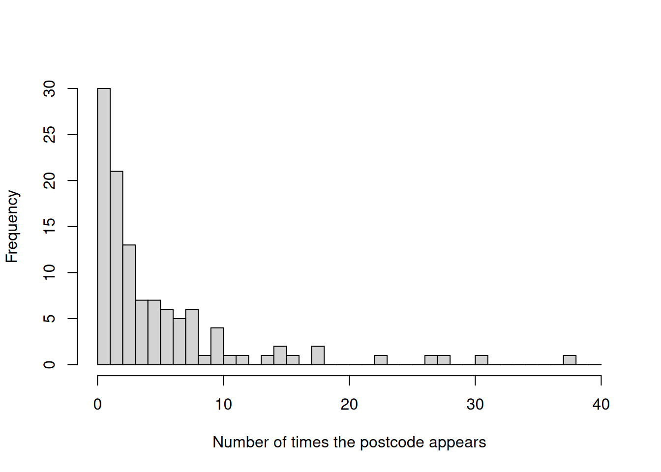
The problem comes with the inclusion of a covariate which is not discussed, and for which no balance statistics are provided. That’s the post-code. This distribution of this variable is very uneven. There is one post-code which features 38 times, and thirty post-codes which only ever appear once.
hist(table(dat$post_code),breaks =0:40,main ="",xlab ="Number of times the postcode appears")
Figure 1: Histogram of postcode frequencies in the data
The analysis depends crucially on the inclusion of this variable. Here I report an analysis which includes education, sex and interior quality, but omits postcode.
Z2 <-model.matrix(~educ + sex + interior_quality -1,data = dat)[,-1]m3 <-rdrobust(y, x, c =0, h =5, b =5,covs = Z2, all =TRUE)summary(m3)
Covariate-adjusted Sharp RD estimates using local polynomial regression.

Number of Obs.                  608
BW type                      Manual
Kernel                   Triangular
VCE method                       NN

Number of Obs.                  446          162
Eff. Number of Obs.             446          162
Order est. (p)                    1            1
Order bias  (q)                   2            2
BW est. (h)                   5.000        5.000
BW bias (b)                   5.000        5.000
rho (h/b)                     1.000        1.000
Unique Obs.                     446          162

=======================================================================================
        Method     Coef. Std. Err.         z     P>|z|      [ 95% C.I. ]
=======================================================================================
  Conventional    -0.205     0.176    -1.170     0.242    [-0.550 , 0.139]
Bias-Corrected    -0.353     0.176    -2.013     0.044    [-0.698 , -0.009]
        Robust    -0.353     0.309    -1.143     0.253    [-0.960 , 0.253]
=======================================================================================
Here, the conventional effect is smaller (-0.2) and no longer statistically significant. The “robust” effect is also not statistically significant. Only the “bias-corrected” effect is statistically significant.
The dependence is specifically a dependence on post-code. When we replaced post-code with the identity of the borough [bezirk], then we don’t get a statistically significant effect either.
### New matrix with `bezname`Z3 <-model.matrix(~educ + sex + interior_quality + bezname -1, data = dat)[,-1]m4 <-rdrobust(y, x, c =0, h =5, b =5,covs = Z3, all =TRUE)summary(m4)
Covariate-adjusted Sharp RD estimates using local polynomial regression.

Number of Obs.                  608
BW type                      Manual
Kernel                   Triangular
VCE method                       NN

Number of Obs.                  446          162
Eff. Number of Obs.             446          162
Order est. (p)                    1            1
Order bias  (q)                   2            2
BW est. (h)                   5.000        5.000
BW bias (b)                   5.000        5.000
rho (h/b)                     1.000        1.000
Unique Obs.                     446          162

=======================================================================================
        Method     Coef. Std. Err.         z     P>|z|      [ 95% C.I. ]
=======================================================================================
  Conventional    -0.190     0.171    -1.111     0.267    [-0.526 , 0.145]
Bias-Corrected    -0.351     0.171    -2.046     0.041    [-0.686 , -0.015]
        Robust    -0.351     0.307    -1.143     0.253    [-0.952 , 0.250]
=======================================================================================
I’ve found it difficult to identify the specific dependence on post-code. When I drop a single post-code at a time, the “robust” results are still significant. The difference between the results cannot therefore be explained as the result of one anomalous post-code.
However, it’s not necessary to identify the specific dependence on post-code to assess the appropriateness of including post-code. As Cattaneo, Idrobo and Titiunik write, to use a RDD with covariates, we need to assume that “the averages of the covariates under treatment and control at the cutoff are equal to each other”; to the extent that that assumption is not met, the design is inappropriate.
Given the distribution of post-codes shown in Figure 1, it should be clear that we can’t demonstrate that the averages of the post-code related covariates are equal to each other at the cut-off. There are thirty post-codes which, because they have only a single value, are necessarily only ever included in the treatment or the control group. There are a further forty-two post-codes which are either all in the treatment condition or all in the control condition. To take the most extreme example: there are 23 respondents from post-code 12439, all of whom are in the control condition.
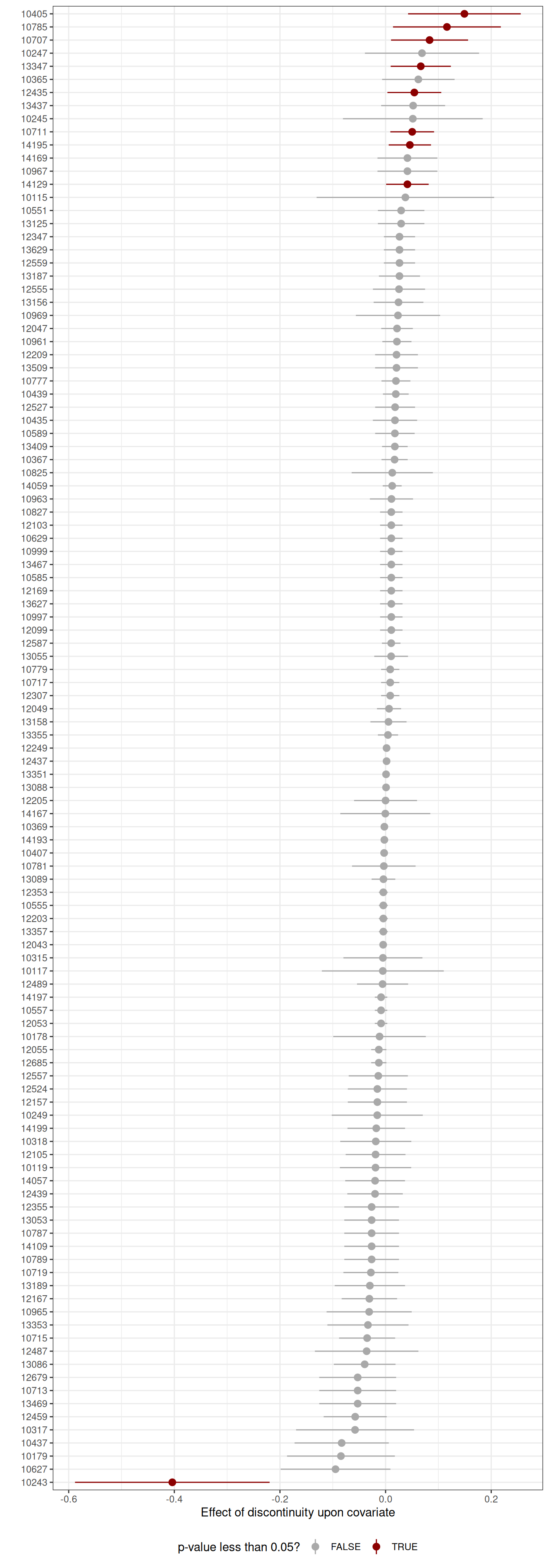
We can, if we wish, proceed to a formal balance check, using the same code that the authors themselves use for their balance figure, Figure A.7 in the appendix. This moves through different outcomes (respondent’s education, apartment quality) and performs a regression discontinuity design using that outcome. If we find a significant treatment effect on that new outcome, we know that there’s imbalance.
Code
# Define a helper functiontidy_rd <-function(model, se_nr) { est <- model$coef[se_nr] se <- model$se[se_nr] low <- model$ci[se_nr, 1] high <- model$ci[se_nr, 2] zstat <- model$z[se_nr] pval <- model$pv[se_nr] h_left <- model$bws[1, 1] h_right <- model$bws[1, 2] b_left <- model$bws[2, 1] b_right <- model$bws[2, 2] p <- model$p n <-sum(model$N_h) smry <-tibble(estimate = est, std.error = se, statistic = zstat,p.value = pval, conf.low = low, conf.high = high, p = p,n = n, bw_left_h = h_left, bw_right_h = h_right, bw_left_b = b_left,bw_right_b = b_right )return(smry)}# Define covariatesoutcomes <-unique(dat$post_code)res <-lapply(outcomes, function(o) { x <- dat |>pull(years_rel_2013) y <-as.numeric(dat$post_code == o) rd <-rdrobust(y = y, x = x, c =0, h =5, b =5)tidy_rd(rd, 3) |>mutate(outcome = o)})res <-bind_rows(res)res <- res |>arrange(estimate) |>mutate(outcome =fct_inorder(outcome))ggplot(res, aes(x = outcome, y = estimate,ymax = conf.low,ymin = conf.high,colour = p.value < .05)) +scale_y_continuous("Effect of discontinuity upon covariate") +scale_x_discrete("") +geom_pointrange() +scale_colour_manual("p-value less than 0.05?",values =c("darkgrey", "darkred")) +coord_flip() +theme_bw() +theme(legend.position ="bottom") res <- res |>mutate(p.adj =p.adjust(p.value, "holm"))
Figure 2: Balance tests for post-codes
As you can see, the discontinuity has significant effects on nine post-codes, of which the largest is the negative effect on 10243 (part of Friedrichshain). What this means is that survey respondents living in buildings built just before 2014, to which the rent control applied, were much less likely to be living in Friedrichshain than survey respondents living in buildings built just after. Yes, this is an odd way of phrasing things.
Obviously one would need to know a lot more either about the history of residential development in Friedrichshain or the survey incentives to give a satisfying account of why this might be. It should be noted, though, that these imbalances are not minor, and achieving a significant imbalance is very hard given the small number of observations for some post-codes. If someone had come to me and said that they were going to run a regression discontinuity on a binary outcome with only 18 positive cases, I would have told them, “go away, your design is hopelessly underpowered”. To give one example: the effect of the previously mentioned post-code 12439, where all 23 respondents are all in the control condition, is not significant.
This suggests to me that although the authors have demonstrated balance with respect to the other categorical covariates included in the model, they have not achieved balance on postcode, and that any model which includes postcode is unsafe.
This criticism comes from inside the regression discontinuity framework, and even more narrowly from the “continuity” approach to regression discontinuity rather than the “local randomization” approach. The continuity approach relies on extrapolation from trends before and after the cut-off. The better we can approximate those trends using a rich and detailed trend line, the better the quality of our inferences. That doesn’t really apply when you have four unique values before your cut-off. It’s hard to draw any trend other that a straight line. Our fancy regression-discontinuity design turns out to be a linear regression in drag. There are alternative approaches to regression discontinuity, such as local randomization, but they typically involve dropping a lot of data.
This ties in to general reservations I have about the use of regression discontinuities where the running variable is a discrete variable which takes on a limited set of values. I think it’s a red flag that rdrobust chokes if you ask it for the “optimal” bandwidth: there’s just not enough data for it to work with. Similarly, RDHonest chokes unless you specify manually the “bound on second derivative of the conditional mean function”.
These software pathologies happen whether or not you control for covariates. Controlling for covariates seems innocuous when it’s presented in textbook treatments – typically applications which rely on huge quantities of administrative data. In these settings, where the data is generally opaque to the people whose outcomes are being modelled, I have no problem with the idea that certain covariates to be pre-treatment. In the survey case, things become slightly more awkward, because people move around. The authors included certain covariates in their pre-analysis plan but removed them from their final analysis because (for example) people might change their party or their apartment size in response to the rent control legislation. If that’s true, why isn’t that true of survey response generally? Would any factor which affects survey response end up being post-treatment? If that’s true, then survey-based regression discontinuity designs with covariates seem like a non-starter.
Footnotes
I don’t know whether reviewers had access to the replication materials.↩︎