tl;dr version

To model the chances of winning a contest, you should use conditional logistic regression, but this requires extra work to turn coefficient values into changes in the probability of winning the contest.

The selection of parliamentary candidates is one of the most important mechanisms in the British political life, yet it’s incredibly hard to research.

That’s why a new paper by Chris Butler, Marta Miori and Rob Ford is so welcome.

The authors compile an anonymized dataset of short-listed candidates, and link candidate characteristics (age, gender, ethnicity) to the chances of being selected as a party candidate.

It’s great work, but that doesn’t mean I wouldn’t like to see some things done differently.

The authors have modelled the probability of success using a logistic regression, where one, or a positive outcome, means being selected, and zero, or a negative outcome, means not being selected.

There are problems with using a logistic regression for this kind of model.

The big problem is that some factors might only matter for selection in a relative sense.

If candidate selection was done by bribery, then all you would need to get selected would be “more bribe money than the other candidate”. In some constituencies – City of London, say – the top bribe might be very high. In other constituencies the top bribe might be very low.

If we just entered the bribe paid by each candidate, we might falsely conclude that the bribe paid had no effect, because some literal losers in City of London paid quite a lot, and some lucky people elsewhere paid very little.

A second problem is that using a logistic regression also complicates making statements about how changes in factors affect the probability of success.

If I change some candidate’s trait – make them male instead of female – then we would like to say that their probability of being selected has gone up – but if we’re saying their probability of being selected has gone up, that implies that the probabilities of selection for other candidates must go down, which wouldn’t happen when you’re generating predictions from a logistic regression.

In this post, I’ll replicate their model using a conditional logistic regression. A conditional logistic regression is exactly the right kind of model when cue Highlander voice there can be only one.

Replicating what was done

I’ll begin by loading the libraries I need, and the replication data. I load tidyverse for general data cleaning, mclogit for modelling. I use modelsummary and hrbrthemes for making stuff look pretty.

set.seed(1891)
suppressPackageStartupMessages({
    library(tidyverse)
    library(mclogit)
    library(modelsummary)
    library(hrbrthemes)
})

dat <- read.delim("ShortlistedCands2019Anonymous.csv",
                  sep = ";",
                  na.strings = c("", "-", "NA"))

I’m going to filter to cases where we know the outcome. I’m also going to create a unique contest identifier, which is created by interacting party and constituency.

dat <- dat |>
    filter(!is.na(success)) |>
    filter(!is.na(BAME)) |>
    mutate(contest = as.numeric(interaction(party, constituency)))

I’ll also remove contests where there was only one candidate listed.

dat <- dat |>
    group_by(contest) |>
    mutate(n_cands = n(),
           pos_within_contest = 1:n()) |>
    ungroup() |>
    filter(n_cands > 1)

I’m also going to drop variables I don’t need:

dat <- dat |>
    dplyr::select(success, contest, gender, BAME, local,
                  past_selection, elected_cllr, occ_party)

Using this, I’ll estimate a model using the same predictors used by the authors to create their Figure 2: being female, being from an ethnic minority, living locally, having stood previously, being an elected councillor, and having worked for the party.

m <- mclogit(cbind(success, contest) ~ gender + BAME + local +
                 past_selection + elected_cllr + 
                 occ_party,
             data = dat)


Iteration 1 - deviance = 265.8233 - criterion = 0.4664284
Iteration 2 - deviance = 265.7618 - criterion = 0.0002312444
Iteration 3 - deviance = 265.7618 - criterion = 1.594636e-08
Iteration 4 - deviance = 265.7618 - criterion = 2.138082e-16
converged

I can then report this model.

my_cm <- c('gender' = 'Female',
        'BAME' = 'Ethnic minority',
        'local' = 'Lives locally',
        'past_selection' = 'Stood before',
        'elected_cllr' = 'Elected councillor',
        'occ_party' = 'Worked for party')
modelsummary(m,
             coef_map = my_cm,
             statistic = "conf.int")

	(1)
Female	-0.531
	[-1.045, -0.017]
Ethnic minority	-0.776
	[-1.564, 0.011]
Lives locally	1.025
	[0.537, 1.513]
Stood before	0.376
	[-0.087, 0.840]
Elected councillor	0.295
	[-0.150, 0.741]
Worked for party	0.255
	[-0.262, 0.772]
Num.Obs.	143
AIC	277.8
BIC	295.5
Log.Lik.	-141.722
RMSE	0.42
nagelkerke's r2	0.245456717189779

Now the coefficient values are there, and you can check how big they are, but it’s quite hard to relate those coefficients – log odds ratios of being chosen – to anything understandable by humans.

We will therefore need to calculate quantities we can understand – like changes in probabilities – under some specific scenarios. Ordinarily, when we calculate human-readable quantities of interest, we calculate average marginal effects, or the effect of changing a focal variable by one unit for each observation, and averaging this over all observations.

A targeted counterfactual

In cases like this, it doesn’t make sense to change the value of the focal variable for one unit for all observations. If the change of one unit affects all observations, then it doesn’t alter the probabilities of success.

We need to therefore consider a more targeted intervention – specifically, what happens if we change the value of the focal variable for a randomly chosen individuals within each contest. We can then average over each of these focal individuals, and calculate the change in the probability for them.

Here’s a function which will take in a data frame, and a variable name contained in a string var and restrict the analysis to contests where there was some variable in the focal variable. It will then randomly choose an individual with the minimum value of the focal variable, alter that individual’s value of the focal variable to the maximum value, and tag that individual as “focal”. This altered variable is stored under the name cfval.

create_counterfactual <- function(data, var) {
    ### Only look at those situations where there is more than one unique value of the variable
    cf <- data |>
        dplyr::ungroup() |>
        dplyr::group_by(contest) |>
        dplyr::mutate(n_distinct = n_distinct(get(var))) |>
        dplyr::ungroup() |>
        dplyr::filter(n_distinct > 1)
    ## set one minimum value to the maximum value
    drop_first <- function(x) {
        x[-1]
    }
    cf <- cf |>
        mutate(randno = rnorm(n())) |>
        dplyr::group_by(contest) |>
        dplyr::arrange(.data[[var]], randno) |>
        dplyr::mutate(cfval = c(max(get(var)), drop_first(get(var))),
                      focal = c(1, rep(0, n() - 1))) |>
        dplyr::select(-randno)
    return(cf)
}

Now that we can create altered sets of data, we need to be able to calculate predicted probabilities. That can be done using the calc_pps function below, which calculates the linear predictor mu, exponentiates it, and divides by the sum of exponentiated predicted probabilities for each contest.

calc_pps <- function(b, X, grp) {
    mu <- X %*% b
    emu <- exp(mu)[,1]
    grpsums <- ave(emu, grp, FUN = sum)
    pr <- emu / grpsums
    return(pr)
}

Finally, we can put this in a overall function, which creates the counterfactuals, does some messing around with model matrices, before drawing some coefficients and calculating averages.

calc_fx <- function(mod, df, var, n_sims = 1000) {
    cf <- create_counterfactual(df, var)

    ### Create the two model matrices
    base_mat <- model.matrix(formula(mod), cf)[,-1]
    newf <- as.character(formula(mod))
    newf <- sub(as.character(var), "cfval", newf)
    newf <- as.formula(paste(newf[[2]], newf[[3]], sep = " ~ "))
    cf_mat <- model.matrix(newf, cf)[,-1]

### Get some betas
    betas <- MASS::mvrnorm(n = n_sims,
                           mu = coef(mod),
                           Sigma = vcov(mod))
    pp <- apply(betas, 1, function(b) calc_pps(b, base_mat, cf$contest))
    cf_pp <- apply(betas, 1, function(b) calc_pps(b, cf_mat, cf$contest))
    delta <- cf_pp - pp
### Just get those comparisons we're interested in
    delta <- delta[which(cf$focal == 1), ]
### Average over cases in the data
    delta <- apply(delta, 2, mean)
### Return the distribution of average effects
    return(delta)
    
}

res <- calc_fx(m, dat, "BAME")

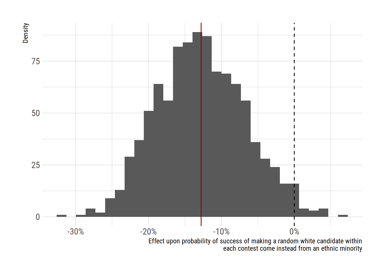
The return value of this function is a vector of n_sims average effect sizes. We can plot the distribution of values like this:

xlab <- str_wrap("Effect upon probability of success of making a random white candidate within each contest come instead from an ethnic minority")
ggplot(data.frame(value = res),
       aes(x = res)) +
    geom_histogram() +
    scale_x_continuous(xlab,
                       labels = scales::percent) +
    scale_y_continuous("Density") +
    geom_vline(xintercept = 0, linetype = 2) +
    geom_vline(aes(xintercept = mean(res)),
               colour = "darkred") + 
    theme_ipsum_rc()

We can see that across multiple simulated batches of coefficients, the average change in probability was -12.8 percentage points. That seems to me to be a pretty major penalty.

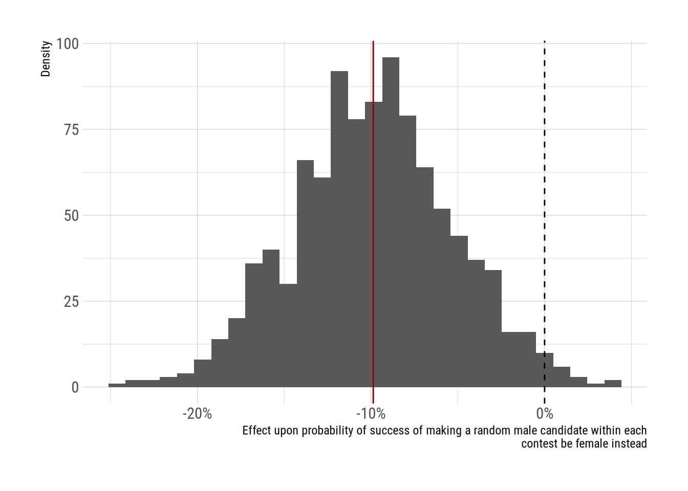
We can repeat this analysis for women candidates. The gender variable is coded so that values of one are equal to women.

res2 <- calc_fx(m, dat, "gender")

xlab <- str_wrap("Effect upon probability of success of making a random male candidate within each contest be female instead")
ggplot(data.frame(value = res2),
       aes(x = res2)) +
    geom_histogram() +
    scale_x_continuous(xlab,
                       labels = scales::percent) +
    scale_y_continuous("Density") +
    geom_vline(xintercept = 0, linetype = 2) +
    geom_vline(aes(xintercept = mean(res2)),
               colour = "darkred") + 
    theme_ipsum_rc()

`stat_bin()` using `bins = 30`. Pick better value with `binwidth`.

Thus, in addition to reporting the coefficient values in their article, the authors might have said:

“changing the gender of a randomly chosen male candidate in a contest to be female is associated with a change in the probability of selection of -9.9 percentage points (95 percent confidence interval: -18.6 to -0.8 percentage points”

and similarly

“making a randomly chosen white candidate in a contest come instead from an ethnic minority is associated with a change in the probability of selection of -12.8 percentage points (95 percent confidence interval: -23.5 to -0.6 percentage points”

both of which are smaller effects than the effects of being local, where they might have said:

res3 <- calc_fx(m, dat, "local")

“making a randomly chosen non-local candidate in a contest come instead from the local area is associated with a change in the probability of selection of 16.9 percentage points (95 percent confidence interval: 9.3 to 23.3 percentage points”

In UK candidate selection, the key really is “location, location, location”…