In the Seat Product Model, the Seat Product is used to bound the number of seat-winning parties, which in turn is used to formulate an expectation regarding the seat share of the largest party. This in turn is used to formulate an expectation regarding the effective number of seat-winning parties: \(N_S = s_1^{-4/3}\). However, the link between the largest share and the effective number is approximate, and it would be good to set it on a firmer footing.

Because I have been reading Jack Bailey’s notes on relationships between effective numbers and Renyi entropy, I got very excited to find a paper bounding Renyi entropies (Gress and Rosenberg 2024) as a function of the size of the largest component. That paper is interested in homozygosity and allele frequency, but maths is maths, right!

In this blog post I show that the bounds in that paper are the same as those identified by Taagepera some years previously, and indeed before any work from Noah Rosenberg on this topic (Rosenberg and Jakobsson 2008). Although these papers are mathematically sophisticated, and are able to construct proofs using majorization, Taagepera got there first (informally, and until some other priority claim rolls in).

Taagepera (2007)

A derivation of the approximation is given in Taagepera (2007), pp. 163–164. I reproduce this here, discussing the upper limit and lower limit separately.

Upper limit

Taagepera writes:

“For a given largest share (\(s_1\)) and number of seat-winning parties (\(N_0\)), the largest possible value of the effective number of parties (\(N\)) corresponds to the other (\(N_0 - 1\)) parties having equal shares \(\tfrac{(1 - s_1)}{(N_0 − 1)}\):”

\[ \max N = \frac{1}{s_1^2 + (N_0 - 1)(1 - s_1)^2 / (N_0 - 1)^ 2} = \frac{1}{s_1^2 + (1 - s_1)^2 / (N_0 - 1)} \]

“As long as \(N_0 = 1/s_1^2\) applies, this expression simplifies into:”

\[ \max N = \frac{1 + s_1}{2 s_1^2} \]

Lower limit

Taagepera writes:

“When \(s_1 = 1/2, 1/3, 1/4\), etc., we can have all shares equal and hence \(N = 1/s_1\). For intervening values of the largest share, making as many shares as possible equal to the largest minimizes \(N\), leaving the remainder as a smaller party.”

Taagepera then presents a set of case-based minima. These minima are expressed solely as a function of \(s_1\), and do not incorporate information about \(N_0\) explicitly (although they may do so implicitly).

Case 1:

“For \(1 < s_1 < 1/2\), no other party can match the largest. The effective number is lowest when the second-largest party is as large as possible, meaning \(s_2 = 1 - s_1\). The resulting minimal effective number is”

\[ \min N = \frac{1}{1 - 2s_1 + 2s_1^2} \]

Case 2:

“For \(1/2 < s_1 < 1/3\), the lowest N corresponds to \(s_2 = s_1\) and \(s_3 = 1 - 2 s_1\). Then”

\[ \min N = \frac{1}{1 - 4 s_1 + 6 s_1^2} \]

Cases 3, 4:

\[ \begin{cases} \min N = \frac{1}{1 - 6 s_1 + 12 s_1^2}, & [1/3 < s_1 < 1/4] \\ \min N = \frac{1}{1 - 8 s_1 + 20 s_1^2}, & [1/4 < s_1 < 1/5] \\ \end{cases} \]

All remaining cases:

\[ \min N = \frac{1}{s_1} \]

Geometric means

Taagepera apparently calculates the geometric mean of these expressions and tries to approximate it. He writes:

“We should try to fit the geometric means of these minimum and maximum values with some simple function of \(s_1\). They can be well fitted with a two-parameter format \(N = a/s1b − a + 1\), which correctly predicts \(N = 1\) when \(s_1 = 1\). The best fit is close to \(N = 2/s_1^{0.9} − 1\). However, we should also try to fit with the simpler one-parameter format \(N = 1/s_1^n\) , because that form can be easily combined with \(s_1 = (MS)^{-1/8}\) so as to connect \(N\) with the seat product \(MS\) in a simple way. This is possible, indeed. Depending on whether one wishes to emphasize the fit at lower or higher values of the largest share, the exponent \(n\) could be taken as anywhere between 1.30 and 1.45. The choice of the simple fraction n = 1/3… agrees with the data”

This implies that if we could find tighter bounds, we could recalculate geometric means, and find some simple approximation. Whether that approximation yielded a better fit would, of course, be an empirical question – but it would be strange if narrower logical bounds yielded worse empirical fit.

Plot

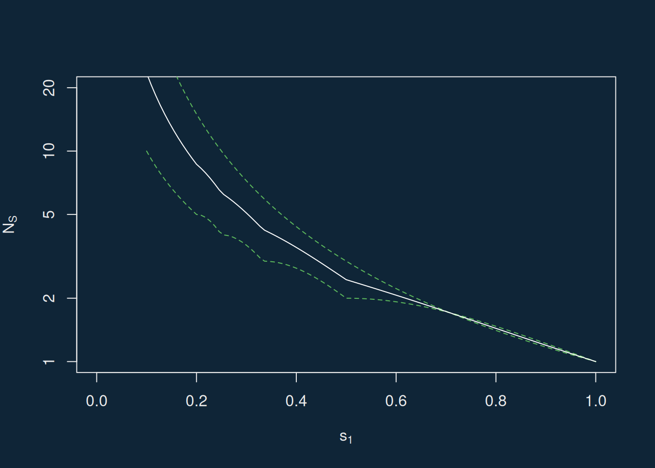
I find understanding these equations hard, so I plot the limits in R.

Code

lb <- function(s1) {
    suppressPackageStartupMessages(require(dplyr))
    case_when(s1 > 1/2 ~ 1 / (1 - 2 * s1 + 2 * s1^2),
              s1 > 1/3 ~ 1 / (1 - 4 * s1 + 6 * s1^2),
              s1 > 1/4 ~ 1 / (1 - 6 * s1 + 12 * s1^2),
              s1 > 1/5 ~ 1 / (1 - 8 * s1 + 20 * s1^2),
              s1 > 0 ~ 1  / s1)
}
ub <- function(s1) {
    (1 + s1) / (2 * s1 ^ 2)
}

par(bg = "#0f2537",
    col.lab = "#ebebeb",
    col.axis = "#ebebeb",
    fg = "#ebebeb")

plot(c(0, 1), c(1, 20), type = "n",
     xlab = expression(s[1]),
     ylab = expression(N[S]),
     log = "y",
     col = "#ebebeb")

inx <- seq(0.1, 1, length.out = 100)
my_lb <- sapply(inx, lb)
my_ub <- sapply(inx, ub)
my_gm <- sqrt(my_lb * my_ub)

lines(inx, my_lb, lty = 2, col = "#5cb85c")
lines(inx, my_ub, lty = 2, col = "#5cb85c")
lines(inx, my_gm, lty = 1, col = "white")

Gress and Rosenberg (2024)

Gress and Rosenberg (2024) set out expressions for lower and upper bounds on the Hill numbers (=effective numbers) of a composition with largest element \(M\) and number of elements \(I\). If we adopt our notation instead, then their expressions are as follows:

\[ N_S \ge \left[ \left \lfloor{1/s_1} \right \rfloor s_1 ^ 2 + (1 - \left \lfloor{1/s_1}\right \rfloor s_1)^2 \right]^{-1/2} \]

and

\[ N_S \le \left[ s_1^2 + (N_{S0} - 1) \left( \frac{1 - s_1}{N_{S0} - 1}\right)^2 \right]^{-1/2} \]

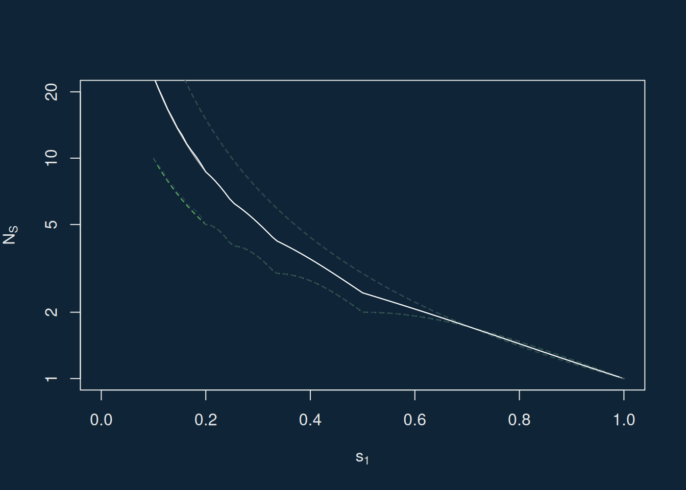
I find it very difficult to look at this formula, and the formulae above, and see whether they’re any different. I’m therefore going to take the dullard’s way, calculating things and then plotting them. I’ll assume \(N_{S0} = 1 / s_1^2\).

Code

lb2 <- function(s1) {
    (floor(1/s1) * s1 ^2 + (1 - floor(1/s1) * s1)^2)^(-1)
}
ub2 <- function(s1) {
    N_S0 <- 1 / s1^2
    (s1^2 + (N_S0 - 1) * ((1 - s1)/(N_S0 - 1))^2) ^ (-1)
}

par(bg = "#0f2537",
    col.lab = "#ebebeb",
    col.axis = "#ebebeb",
    fg = "#ebebeb")

plot(c(0, 1), c(1, 20), type = "n",
     xlab = expression(s[1]),
     ylab = expression(N[S]),
     log = "y")

inx <- seq(0.1, 1, length.out = 100)
my_lb2 <- sapply(inx, lb2)
my_ub2 <- sapply(inx, ub2)
my_gm2 <- sqrt(my_lb2 * my_ub2)

lines(inx, my_lb, lty = 2, col = "#5cb85c")
lines(inx, my_ub, lty = 2, col = "#5cb85c")
lines(inx, my_gm, lty = 1, col = "grey")

lines(inx, my_lb2, lty = 2, col = "#2b3e50")
lines(inx, my_ub2, lty = 2, col = "#2b3e50")
lines(inx, my_gm2, lty = 1, col = "white")

Here the two sets of bounds overlap perfectly, and so whilst the expression found in Gress and Rosenberg (2024) is neater, it doesn’t help us advance on Taagepera (2007).

Conclusion

Sometimes I am easily impressed by papers which look complicated, but which don’t yield advances in knowledge.

References

Gress, Theodore D, and Noah A Rosenberg. 2024. “Mathematical Constraints on a Family of Biodiversity Measures via Connections with rényi Entropy.” BioSystems 237: 105153.

Rosenberg, Noah A, and Mattias Jakobsson. 2008. “The Relationship Between Homozygosity and the Frequency of the Most Frequent Allele.” Genetics 179 (4): 2027–36.

Taagepera, Rein. 2007. Predicting Party Sizes: The Logic of Simple Electoral Systems. OUP Oxford.