Some relationships are linear. If I work eight hours and make eight widgets, then an extra hour’s work will probably give me one more widget.
We could pick apart this example. You might suggest that I’ll be tired at the end of a working day, and will be lucky to squeeze out that extra widget. You might be right. You might also challenge the fascination with widgets found in economics texts. Here too you would also be right. Permit me the example.
Other relationships are nonlinear. This includes lots of relationships involving growth. A particular technology might expand from 25,000 to 50,000 users in the course of a month, and then expand from 50,000 to 100,000 users in the course of the next month. “One extra month” yields a different number of additional users depending where we are on the growth curve.
In the social sciences, we tend to think of relationships as linear. This in part is because many of the tools we use to model relationships are linear, or linear in parameters. Most regression models are (generalized) linear models.
Even when we predict nonlinear relationships, we often transform them so that they become linear. In the subfield I know best, one “basic law” from the Seat Product Model is that the effective number of seat-winning parties is equal to the seat product \(MS\) raised to the power of one-sixth:
\[
N_S = (MS)^{\tfrac{1}{6}}
\tag{1}\]
However, the regression model that is used to test this relationship is a linear model:
\[
log(N_S) = a + k \cdot \log(MS)
\tag{2}\]
which takes advantage of the way logarithms turn multiplication into addition. If Equation 1 is correct, then we would expect \(a = 0, k
= \tfrac{1}{6}\).
Social scientists are not alone in turning nonlinear relationships into linear relationships for the purposes of statistical testing. Allometry is a subfield of biology which deals with relationships between sizes (and sometimes rates) of animals. Lots of allometric relations follow Equation 1, but are tested using Equation 2. Packard (2014) describes this as the “traditional method” of estimating such relationships.
What is wrong with linearizing relationships?
Sweet summer children might believe that linearizing relationships cannot have any harmful consequences if it is so widely used. However, whenever we take logarithms we’re changing the type of mean we predict. In an ordinarily least squares regression, we’re predicting an average arithmetic mean. If we’re working on the log transformed scale, we’re still predicting an average arithmetic mean, but on the log scale. That means that when we reverse the log operation, the mean we get back will be smaller than the mean of the original, un-transformed data.
Table 1: Example of transformation bias taken from Smith (1993)
Original data
Base 10 log transformed data
1.0
0
10.0
1
100.0
2
1000.0
3
Mean
10000.0
4
2222.2
2
Table 1 an example from Smith (1993). We have a set of numbers which range from one to ten thousand. Their average is a little over two thousand. Because these numbers are all positive, and span a couple of orders of magnitude, we might think to log-transform them. Here I’ll use log to the base 10 to keep the numbers simple. We might then estimate an intercept-only regression on the log-transformed values to get a mean. The mean of the log-transformed values is just 2, and when we back-transform we get \((10^2 =) 100\), far less than the mean we “ought” to get.
The response to this “transformation bias” is very much to suggest that this theoretical problem is not a practical problem. Xiao et al. (2011) collect a large number of allometric datasets and fit models to them using the traditional method of log transformation and by using nonlinear least squares fits. The conclusion is that, for two thirds of data-sets, the fit between the model and data was better with a log-transformed model than with a nonlinear least squares model.
Additive and multiplicative error
Not everyone is convinced that the old ways are best. Gary Packard, who as far as I can tell has been waging a one-man battle against logarithmic transformations for allometry, argues that Xiao et al. (2011) make nonlinear regression look bad, because they assume that nonlinear regression modelling uses additive error, and that when nonlinear regression uses multiplicative error it looks much better.
What do I mean by additive or multiplicative error? I can explain it best by starting with the log transformed equation
\[
\log(y) = a + k \log(x) + \epsilon
\]
where the error terms epsilon come from some normal distribution with a mean of zero and an estimated standard deviation \(\sigma\).
\[
\epsilon \sim N(0, \sigma^2)
\]
In this equation, the error term \(\epsilon\) is additive on the log-transformed scale. By additive, I just mean, “we add it on”, even though when we add on negative errors it is more natural to talk of subtraction.
However, when the error on log-transformed scale is additive, the error is multiplicative on the original scale. In order to show this, we exponentiate everything in the above equation to get
\[
y = ax ^ k \exp(\epsilon)
\]
Here, any positive or negative values of \(\epsilon\) are exponentiated, and multiply the term \(ax ^ k\). Instead of adding or subtracting some error from our prediction, we scale it up or down by some factor.
Multiplicative error seems more appropriate when dealing with outcomes than span several orders of magnitude. Suppose we were dealing with deaths in wars. In some wars dozens of people die; in other wars millions of people die. Being able to predict war deaths “plus or minus a thousand” would be ridiculous in the case of a conflict which we predicted to involve a dozen deaths, and spuriously precise in cases where we predict millions of deaths.
Unfortunately, most nonlinear regression routines in statistical software don’t estimate multiplicative error. The variance structure recommended by Packard, and which is implemented in some R routines, is to set error proportional to the predicted value, raised to some power:
\[
y \sim N(a x^k,
\sigma^2 \cdot (a x ^ k)^{2\delta})
\]
where \(\delta\) is a parameter to be estimated, and where values greater than zero indicate that variance increases proportionate to the predicted value. A value of zero for \(\delta\) implies constant additive variance on the original scale. Packard refers to this as additive heteroscedastic error, which is true in the sense that the error is added on, but confusing in the sense that the \(\sigma\) term here is clearly multiplying \(ax^k\).
Worked example (1)
Let’s see how this might work in practice. I’m going to work with data from electoral studies, and specifically the National and District Level Party System Datasets described in Struthers et al. (2018). I’ll use this data to test some claims made by the Seat Product Model, as set out in Shugart and Taagepera (2017).
I begin by loading the libraries I need – haven for file import, modelsummary to show the results of my regressions, and nlme for the modelling.
I’ll then load in the data, and filter only to simple (i.e., single ballot, single tier, non-preferential) electoral systems where we know the seat product, or the average district magnitude times the assembly size.
I’m going to begin with an example where three different methods reach the same conclusion. That is, I’m going to test the claim that the effective number of seat-winning parties is equal to the seat product, raised to the power of one sixth.
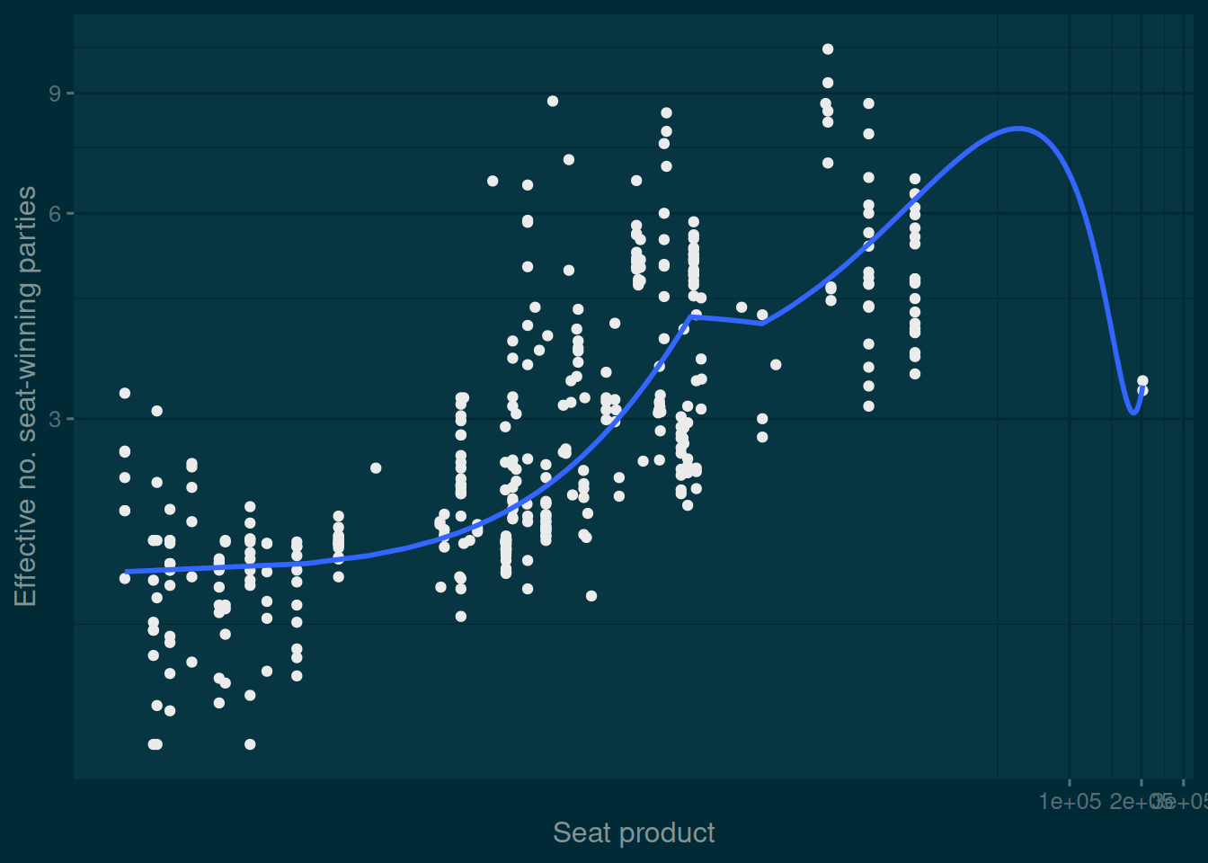
Let’s test the most basic claim, that the effective number of seat-winning parties is related to the seat product. We can (and should!) visualize these variables before we do anything else. Here I’ll use log-transformed axes, without by this implying any commitment to log transforming the variables in the regressions I’ll run shortly.
The outlier to the right is Ukraine between 2006 and 2007, where the effective number of parties is low but where there were a tonne of independents.
Code
m <-lm(log(Ns) ~log(seat_product), data = dat)my_cm <-c("(Intercept)"="Constant","log(seat_product)"="log(Seat product)")modelsummary(m,coef_map = my_cm,statistic ="conf.int",gof_map =c("nobs", "r.squared"))
Table 2: Log log regression of the effective number of parties on the seat product.
(1)
Constant
-0.012
[-0.112, 0.087]
log(Seat product)
0.165
[0.150, 0.180]
Num.Obs.
403
R2
0.538
We find that everything works – the confidence interval for our constant includes zero, and the confidence interval on the logged seat product includes one-sixth. We seem to be in the world described by Xiao et al. (2011), where log transforming “just works”.
We can now try modelling things in nls, R’s default routine for nonlinear least squares. This uses additive error, and so wouldn’t be recommended by Packard. As with all invocations of nls, we have to provide some starting values for the parameters, but with a relatively simple model these are innocuous.
Table 3: Nonlinear least squares regression of the effective number of parties, additive error.
(1)
(2)
k
0.170
0.158
[0.165, 0.174]
[0.140, 0.177]
a
1.097
[0.937, 1.257]
Num.Obs.
403
403
Despite the (probably incorrect) use of additive error , everything seems to work as it did before. In the first model, which uses just the exponent \(k\), the confidence interval includes one-sixth, even though it’s somewhat on the high side. In the second model, which includes an additional term to match the two term log log models just discussed, the confidence interval on the extra term includes \(\exp(0)
= 1\), which is as it should be.
Finally, let’s try modelling it in nlme, with variance proportional to a power of the predicted value.
Code
m3 <-gnls(Ns ~ seat_product ^ k, data = dat,start =list(k =1/2),weights =varPower(form =~fitted(.)))m3b <-gnls(Ns ~ a * seat_product ^ k, data = dat,start =list(a =1, k =1/2),weights =varPower(form =~fitted(.)))modelsummary(list(m3, m3b),statistic ="conf.int",gof_map =c("nobs", "r.squared"))
Table 4: Nonlinear least squares regression of the effective number of parties, error proportional to predicted value.
(1)
(2)
k
0.171
0.166
[0.165, 0.176]
[0.149, 0.183]
a
1.033
[0.925, 1.141]
Num.Obs.
403
403
R2
0.429
0.431
Now in the two parameter model the exponent \(k\) is exactly what it was predicted to be, to three decimal places. What the modelsummary output doesn’t show is the parameter \(\delta\), which is estimated to be somewhat greater than one, suggesting that error is slightly greater when we reach higher values of the seat product.
Worked example (2)
So far, so boring – modelling the relationship in three different ways gives substantially the same results. That might be a signal that we’ve found a robust relationship, but equally it might be sign that we are spending time on modelling details that don’t matter. What about an example where the three methods give different results?
We can stick with the same data-set, and model not the effective number of seat-winning parties but rather the raw number. The claim made by Shugart and Taagepera (2017) is that the raw number of seat-winning parties should be equal to the seat product to the power of one quarter. Taagepera and Shugart actually make their prediction about the effective number only after making a prediction for the raw number – so if these worked examples recapitulated the theoretical order of the claims, we should have started here with the raw number.
Let’s start with taking logs on both sides.
Code
m <-update(m, log(Ns0) ~ .)modelsummary(m,coef_map = my_cm,statistic ="conf.int",gof_map =c("nobs", "r.squared"))
Table 5: Log log regression of the effective number of parties on the seat product.
(1)
Constant
0.114
[-0.058, 0.286]
log(Seat product)
0.238
[0.212, 0.264]
Num.Obs.
403
R2
0.448
So far so good – we have an intercept which could be zero, and a coefficient which could be one quarter, as predicted.
What about nonlinear least squares with additive error?
Table 6: Nonlinear least squares regression of the raw number of parties, additive error.
(1)
(2)
k
0.258
0.159
[0.247, 0.268]
[0.119, 0.200]
a
2.373
[1.610, 3.137]
Num.Obs.
403
403
Here something seems to have come off the rails. Although the single parameter model conforms to expectations, in the sense that the value of \(k\) could be one quarter, the two parameter model has a value of \(k\) that is far too low.
Can we rescue this – and nonlinear least squares – by incorporating error that is proportionate to the predicted value?
Code
m3 <-gnls(Ns0 ~ seat_product ^ k, data = dat,start =list(k =1/2),weights =varPower(form =~fitted(.)))m3b <-gnls(Ns0 ~ a * seat_product ^ k, data = dat,start =list(a =1, k =1/2),weights =varPower(form =~fitted(.)))modelsummary(list(m3, m3b),statistic ="conf.int",gof_map =c("nobs", "r.squared"))m3 <-gnls(Ns0 ~ seat_product ^ k, data = dat |>filter(seat_product <1e5),start =list(k =1/2),weights =varPower(form =~fitted(.)))m3b <-gnls(Ns0 ~ a * seat_product ^ k, data = dat |>filter(seat_product <1e5),start =list(a =1, k =1/2),weights =varPower(form =~fitted(.)))modelsummary(list(m3, m3b),statistic ="conf.int",gof_map =c("nobs", "r.squared"))
Table 7: Nonlinear least squares regression of the raw number of parties, error proportional to prediction.
(1)
(2)
k
0.282
0.237
[0.268, 0.296]
[0.192, 0.281]
a
1.373
[0.963, 1.784]
Num.Obs.
403
403
R2
0.033
0.109
(1)
(2)
k
0.283
0.245
[0.269, 0.297]
[0.199, 0.290]
a
1.311
[0.916, 1.706]
Num.Obs.
401
401
R2
0.109
0.149
In model (2), the value of \(k\) is once against consistent with the predicted value of one quarter, and the value of \(a\) is (just) consistent with a value of one. Thus, although a log log regression gave the “right” answer, and one nonlinear regression gave the “wrong” answer, that was because when we estimate a nonlinear regression we have to get our error structure right.
Conclusions
In the worked examples I’ve set out, I was modelling numbers of parties, something that doesn’t vary over more than one order of magnitude.
The issues with fixed exponent relationships of the form \(y = a x ^ k\) are likely to be more severe when dealing with data like conflict deaths which do range over orders of magnitude.
As always, we need to think carefully about our errors, and use the appropriate tools for the job. Generally, social scientists don’t think enough about variance (Braumoeller 2006), but that’s something that we’re forced to do when we step into nonlinear modelling.
References
Braumoeller, Bear F. 2006. “Explaining Variance; or, Stuck in a Moment We Can’t Get Out Of.”Political Analysis 14 (3): 268–90.
Packard, Gary C. 2014. “On the Use of Log-Transformation Versus Nonlinear Regression for Analyzing Biological Power Laws.”Biological Journal of the Linnean Society 113 (4): 1167–78.
Shugart, Matthew S, and Rein Taagepera. 2017. Votes from Seats: Logical Models of Electoral Systems. Cambridge University Press.
Smith, Richard J. 1993. “Logarithmic Transformation Bias in Allometry.”American Journal of Physical Anthropology 90 (2): 215–28.
Struthers, Cory L, Yuhui Li, and Matthew S Shugart. 2018. “Introducing New Multilevel Datasets: Party Systems at the District and National Levels.”Research & Politics 5 (4): 2053168018813508.
Xiao, Xiao, Ethan P White, Mevin B Hooten, and Susan L Durham. 2011. “On the Use of Log-Transformation Vs. Nonlinear Regression for Analyzing Biological Power Laws.”Ecology 92 (10): 1887–94.